Animation Easing in OpenSCAD

OpenSCAD provides a $t variable as a representation of the animation’s progress. It starts at 0, increases to 1, and immediately loops back to 0. The movement is called linear because each step is equal across the timeline.

Things in real life, however, hardly ever move exactly linearly. Consider a bouncing ball or a felled tree or your swaying arms as you walk. Gravity accelerates each, increasing its speed as it falls; if it comes back up, like the ball or a swaying arm, it decelerates to zero velocity at the apex when the cycle repeats.

Motion designers call the math of how an object moves between two states an easing function. I won't pretend to fully understand how they all work mathematically, but I luckily don't have to; because their definitions don’t change across different programming languages, porting from one to another is relatively straightforward.

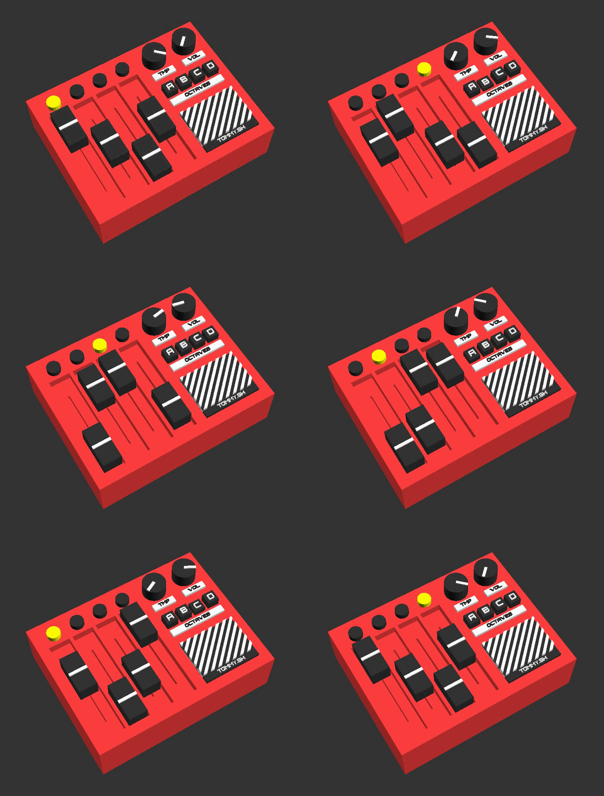
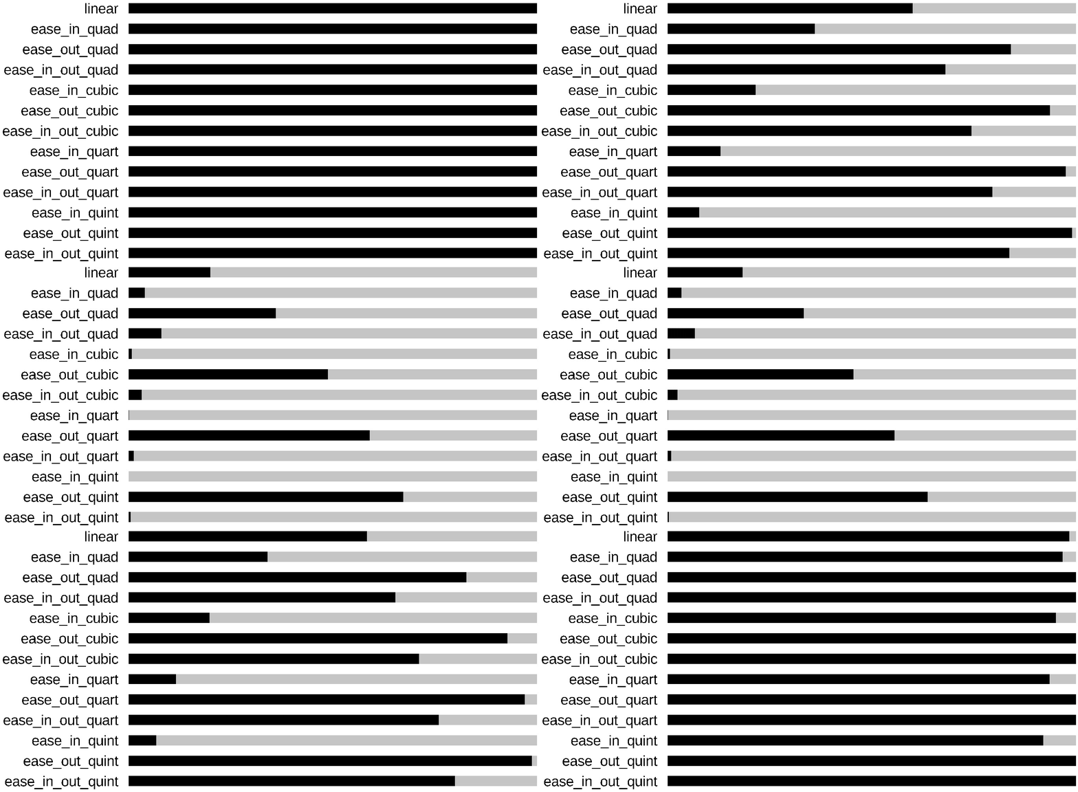
Demo

Code

(Demo code available here. Based on Easing Equations by Robert Penner.)

Usage

Simply include the file and wrap $t in any of its functions.

include <easing-functions.scad>;

translate([ease_in_cubic($t) * x, 0, 0]) { ... }
rotate([0, 0, 360 * ease_in_out_cubic(undulate($t)]) { ... }

Unless the starting and finishing states are identical (like cyclically rotating from 0 to 360 degrees), you’ll want a timing variable that fully goes back and forth, from 0 to 1 and back down to 0. The demo above does this by doubling the absolute distance from the midpoint:

function undulate(t) = abs((t - .5) * 2);

In the end, it may seem like an oxymoron to fret over realism in CAD software specifically designed more for machine parts than lifelike art, but I've found that if it's a trivial amount of effort to make any artificial thing more believable as a real thing, it's worth it.